How to quantize models with 16-bit activations (W8A16 Qmn)
How to quantize models with 16-bit activations (W8A16 Qmn)

This tutorial shows how to quantize a float ONNX model to
W8A16 Qmn
(8-bit weights,
16-bit activations, power-of-two scales) with the ST fork of
AMD Quark, an open-source quantization toolkit for
PyTorch and ONNX models. It also shows how to check on a PC that the quantized model keeps the
accuracy of the float model. It covers an
image classification
use case (Python script) and
a
time-series regression
use case (Jupyter notebook). It uses AMD Quark directly, without
STM32 Model Zoo Services.
Generate a
W8A16 Qmn quantized ONNX model
from a float ONNX model, and
compare its
accuracy with the float model
on a PC, for two use cases:
Image classification: an FD-MobileNet classifier from the STM32 Model Zoo, trained on
the Flowers dataset, quantized and evaluated with a Python script.
Time-series regression: a 1D convolutional altitude regressor, trained, quantized, and
evaluated in a Jupyter notebook.
Note
This tutorial covers
quantization and host evaluation only. It runs on a Windows or
Linux PC, on CPU. Deploying the quantized model on an STM32 target is out of scope.
A C++ build toolchain, because Quark compiles its custom operators the first time it
runs: the Microsoft C++ Build Tools on Windows (see 1. Install the C++ build tools), GCC on
Linux.
The tutorial files (scripts, float model, notebook, and helper module), see
Assets.
Quantization represents each real value as an integer multiplied by a
scale
(real value ≈ integer value × scale).
Calibration
chooses the activation scales, by
running representative input data through the float model.
W8A16
keeps the
weights in 8-bit
integers and quantizes the
activations to 16-bit
integers. Compared with the common
W8A8
scheme, 16-bit activations reduce the quantization
noise in intermediate tensors, at the cost of larger activation buffers.
Qmn
restricts every scale to a
power of two. Each quantized value is then a signed
fixed-point number in the Qm.n format: 1 sign bit,
m
integer bits, and
n
fractional bits.
Real value = integer value × 2⁻ⁿ. There is no zero-point: the quantization is symmetric.
Example: in the Q3.12 format, a 16-bit activation covers -8 to +7.9998, with a resolution
of 2⁻¹² ≈ 0.00024.
Benefit: rescaling between layers becomes a bit shift, which suits fixed-point integer
arithmetic.
Trade-off: power-of-two scales offer fewer choices than float scales, which can add
quantization error.
AdaQuant
is an optional post-training step. After calibration, it fine-tunes the
weights and biases
of each quantized layer on the calibration data, to reduce the
difference between the layer output and the float layer output. The scales chosen by the
calibration do not change. AdaQuant often reduces the accuracy loss, but it does not
guarantee better test metrics, and more iterations increase the quantization time.
In AMD Quark, a
quantization spec
class sets the integer type, the scale type, and the
calibration method of a tensor:
XInt8Spec and XInt16Spec: power-of-two scales (Qmn), MinMSE calibration. The ST
fork adds the XInt16Spec class, required for 16-bit Qmn activations.
Int8Spec and Int16Spec: float scales, Percentile calibration. Int8Spec
gives the standard W8A8 quantization.
This tutorial uses
XInt8Spec
for the weights. To compare 16-bit with 8-bit activations,
it uses
XInt8Spec
for the activations too (
W8A8 Qmn): only the activation width
changes.
Run the Build Tools installer. If the Build Tools are already installed, open the
Visual Studio Installer and click Modify on the Build Tools.
Check Desktop development with C++.
In the Installation details panel, check that MSVC x64/x86 build tools and a
Windows 11 SDK are selected.
Click Install (or Modify).
To add the workload to installed Build Tools from the command line, run the following
command in a PowerShell run as administrator. Replace the --installPath value with the
folder of your Build Tools, given by
&'C:\ProgramFiles(x86)\MicrosoftVisualStudio\Installer\vswhere.exe'-products*-propertyinstallationPath.
On Windows, run the commands of Part 1 from the
x64 Native Tools Command Prompt for
VS
(Start menu, Visual Studio folder). This prompt puts the 64-bit C++ compiler
(
cl.exe) on the
PATH. The
Developer Command Prompt for VS
sets up the 32-bit
compiler instead.
Quark compiles its custom operators only once, in step 5, and caches them in
%LOCALAPPDATA%\torch_extensions. After that, you can use any terminal.
If the compilation still fails on Windows, the Windows Subsystem for Linux (WSL) is an
alternative: follow the Linux instructions in WSL.
Quark supports
Python 3.11, 3.12, and 3.13. This tutorial was tested with Python 3.13:
with Python 3.11 or 3.12, replace
3.13
in the commands below.
Open a terminal in your working folder: on Windows, the x64 Native Tools Command Prompt
for VS.
Create and activate the virtual environment.
Windows (Command Prompt):
py -3.13 -m venv .venv
.venv\Scripts\activate.bat
Linux:
python3.13-mvenv.venv
source.venv/bin/activate
In PowerShell, activate the environment with .venv\Scripts\Activate.ps1. If
PowerShell blocks the script, run Set-ExecutionPolicy-ScopeCurrentUserRemoteSigned
once, then activate the environment again.
Upgrade the packaging tools:
python-mpipinstall--upgradepipsetuptoolswheel
Important
Keep the virtual environment
activated
for all the commands of this tutorial. Quark
also needs the
ninja
build tool, which is installed in the virtual environment.
--no-build-isolation makes pip build Quark with the PyTorch version of the virtual
environment. Without this option, pip builds Quark with the latest PyTorch release, which
fails on Windows. The installation takes a few minutes: pip also installs the
dependencies of Quark.
Important
Do not install
amd-quark
from PyPI in this environment: the PyPI release does not
provide
XInt16Spec.
The first command prints Version:0.12.post1+9d632d9 for the tested commit, and an
Editableprojectlocation in the AMD-Quark clone.
The second command compiles the Quark custom operators, in less than a minute. Its log
must contain:
[QUARK-INFO]: CPU version of custom ops library compiled successfully (JIT fallback).
Or, when the custom operators are already compiled:
[QUARK-INFO]: The CPU version of custom_ops library already exists at ...
The second command ends with XInt16Specavailable.
Warning
XInt16Spec


                available
is printed even if the compilation of the custom operators
fails. Always check the log: if it contains
CPU


                version


                of


                custom


                ops


                library


                compilation


                failed
, see
Troubleshooting.
Note
Before the compilation, a warning reports that the custom ops library does NOT exist: this
is expected. The
PyTorch


                2.7.1+cpu:


                skipping


                stable-ABI


                pass


                (requires


                >=


                2.10)
message is harmless. With a CUDA build of PyTorch, Quark also tries to compile a GPU
version of the custom operators: if this compilation fails, quantization still runs on
CPU.
In this part, the
qmn_adaquant_image_classification_tutorial.py
script quantizes a float
ONNX image classifier to W8A16 Qmn, then compares the top-1 accuracy of the float and
quantized models on a labeled test set.
The example model is the
FD-MobileNet α = 0.25
classifier of the STM32 Model Zoo
(224×224 RGB inputs), trained on the
Flowers
dataset: 3670 photos of 5 classes (daisy,
dandelion, roses, sunflowers, and tulips).
Download the following files to your working folder (see Assets):
qmn_adaquant_image_classification_tutorial.py: the quantization and evaluation
script
prepare_flowers_dataset.py: the dataset preparation script
fdmobilenet_a025_224_tfs_float32.onnx: the float model
Prepare the datasets:
pythonprepare_flowers_dataset.py
The script downloads and extracts the Flowers dataset (218 MB), then creates the
datasets folder:
datasets/
├── calibration/     # 200 images of the training split
│   ├── daisy/
│   └── ...
└── test/            # 734 images, one sub-folder per class
    ├── daisy/
    ├── dandelion/
    ├── roses/
    ├── sunflowers/
    └── tulips/
The test set is the validation split of the Model Zoo training (20 % of the images, seed
127): the model never saw these images during training. The calibration images come from the
training split.
The float model is the
.keras
model of the Model Zoo, converted to ONNX with
tf2onnx
(opset 17), with an NCHW input:
batch×3×224×224.
To use
your own model and dataset, provide:
Input
Requirements
Float ONNX model
Float32 classifier with a
single NCHW input
and one score per class as output
Calibration images
Representative images
(
.jpg,
.jpeg, or
.png) in one folder, searched
recursively. Labels are not needed. Take them from the training data, never from the
test set. A few hundred images is a good starting point.
Test images
Labeled images, in one sub-folder per class
Warning
The script numbers the classes in the
alphabetical order of the test sub-folder names
(torchvision
ImageFolder
convention). This order must match the class order used to
train the model, otherwise the measured accuracy is wrong. For the Flowers model, the
class order of the Model Zoo is alphabetical.
The calibration and test images must be preprocessed exactly like the training images. The
script applies the same
build_transform()
function to both:
defbuild_transform(input_size:int=224,interpolation:str="bilinear")->torchvision.transforms.Compose:"""Preprocessing shared by calibration and evaluation: it must match the training preprocessing."""returntorchvision.transforms.Compose([torchvision.transforms.Resize((input_size,input_size),interpolation=torchvision.transforms.InterpolationMode(interpolation),),torchvision.transforms.ToTensor(),# RGB, HWC -> CHW, [0, 255] -> [0.0, 1.0]torchvision.transforms.Normalize(mean=[0.5,0.5,0.5],std=[0.5,0.5,0.5]),# -> [-1.0, 1.0]])
The FD-MobileNet Flowers model expects RGB images, resized to 224×224, with pixel values in
[-1, 1]. If your model uses another preprocessing (color order, normalization, input size, or
resize method),
update this function, or use the
--input-size
and
--interpolation
arguments: a mismatch degrades both the calibration and the measured
accuracy.
Quark reads the calibration data through a
calibration data reader. In the script, the
ImageDataReader
class preprocesses the calibration images with
build_transform(). Its
get_next()
method returns one preprocessed image per call, as an
{input_name:


               array}
dictionary, and
None
when all images have been read.
Check the preprocessing before quantizing: evaluate the float model only, with the
--float-only
argument. This takes a few seconds, whereas the quantization takes a few
minutes.
Expected result:Float
accuracy:
0.8202. A much lower accuracy reveals a
preprocessing mismatch: for example, with pixel values in [0, 1] instead of [-1, 1], the
accuracy of this model drops to 0.4768.
Note
The Model Zoo trained this model with nearest-neighbor resizing. With
--interpolationnearest, the float accuracy is 0.8147, slightly lower: this
tutorial keeps the default bilinear resizing.
The script keeps all calibration images in memory, as float32 arrays: about 0.6 MB per
224×224 image.
The
build_qmn_config()
function of the script builds the Quark configuration:
weight_spec=XInt8Spec()weight_spec.set_quant_granularity(QuantGranularity.Channel)activation_spec={8:XInt8Spec,16:XInt16Spec}[activation_bits]()algorithms=[]ifadaquant:algorithms.append(AdaQuantConfig(learning_rate=1e-5,num_iterations=num_iterations))returnQConfig(global_config=QLayerConfig(activation=activation_spec,weight=weight_spec),algo_config=algorithms,extra_options={# Keep Clip (ReLU6) and ReLU after convolutions, with their Q/DQ nodes"ConvertClipToRelu":False,"RemoveQDQConvClip":False,"RemoveQDQConvRelu":False,},OpTypesToQuantize=None,QuantizeBias=True,CalibMovingAverage=False,AlignSlice=False,FoldRelu=True,AlignConcat=True,EnableNPUCnn=False,)
Setting
Effect
XInt8Spec()
with
QuantGranularity.Channel
8-bit symmetric weights, one power-of-two scale
per output channel
XInt16Spec()
16-bit symmetric activations, one power-of-two scale
per tensor. With
--activation-bits


                    8
, the script uses
XInt8Spec()
instead (W8A8 Qmn).
Calibration method
MinMSE, the default of both specs: selects the power-of-two scale that minimizes
the mean squared quantization error on the calibration data
AdaQuantConfig
Enables AdaQuant, with a learning rate of
1e-5.
num_iterations
is the number
of iterations
per layer
(500 by default in the script).
ConvertClipToRelu,
RemoveQDQConvClip, and
RemoveQDQConvRelu
set to
False
Keep the Clip (ReLU6) and ReLU activations after the convolutions, with their Q/DQ nodes
QuantizeBias=True
Quantizes the biases
EnableNPUCnn=False
Disables the quantization constraints specific to AMD NPUs
Graph and calibration options of the Quark power-of-two flow: keep the example values
Note
The time-series notebook of Part 3 uses the same settings, with 100 AdaQuant iterations,
QuantizeAllOpTypes=True
(all operator types are quantized), and Q/DQ nodes also kept
after LeakyRelu and PRelu activations.
In the Windows Command Prompt, write the command on a single line, or replace each
\
with
^. In PowerShell, replace each
\
with a backtick (
`).
The script checks the paths, then runs three stages:
Float evaluation: ONNX Runtime computes the top-1 accuracy of the float model.
Calibration and quantization: Quark calibrates the scales, runs AdaQuant layer by
layer, and saves the W8A16 Qmn model.
Quantized evaluation: ONNX Runtime computes the top-1 accuracy of the quantized model.
Note
The script takes about 3 minutes on a laptop CPU. Most of this time is the
MinMSE
calibration of the activations: about 2 minutes for 200 calibration images, growing with
the number of images. AdaQuant (500 iterations per layer) takes about 30 seconds.
Optional arguments:
Argument
Description
--float-only
Evaluates the float model only, to check the preprocessing.
--quantized-model
and
--calib-dir
are then not needed.
--activation-bits
16
for W8A16 Qmn (default),
8
for W8A8 Qmn
--input-size
Square input resolution of the model (default:
224)
--interpolation
Resize method:
bilinear
(default) or
nearest
--batch-size
Evaluation batch size (default:
32). Use
1
if the batch dimension of the model
is fixed.
At the end of the quantization, Quark prints a table of the quantized operator types, with
INT16 activations, and INT8 weights for the 24 convolutions.
The quantized model is saved to the --quantized-model path. It is an ONNX model in
QDQ format: 42 QuantizeLinear and 90 DequantizeLinear nodes of the
com.microsoft domain carry the int8 and int16 quantization parameters. The model
inputs and outputs stay float32. The file size is about 230 kB, versus 513 kB for the float
model.
The script ends with the accuracy comparison on the 734 test images:
Reference results with the other configurations of the script:
Configuration
Top-1 accuracy
Accuracy drop
Run time
Float model
82.02 %
—
—
W8A16 Qmn with AdaQuant (default)
81.88 %
0.14 points
3 min
W8A16 Qmn without AdaQuant (
--no-adaquant)
82.29 %
-0.27 points
2 min
W8A8 Qmn with AdaQuant (
--activation-bits


                    8
)
81.88 %
0.14 points
2.5 min
On 734 test images, one image represents 0.14 points: a difference of a few images is
noise. A negative accuracy drop, where the quantized model is slightly better, is noise
too.
On this classifier, W8A16 and W8A8 give the same accuracy: the classifier is robust to
8-bit activations. Part 3 shows a regression model where 16-bit activations make a clear
difference.
Your values can differ slightly, depending on your platform and package versions. Compare
the accuracy drop with the accuracy loss acceptable for your application. If the drop is too
large, see
Troubleshooting.
Part 3 — Quantize a time-series regression model

In this part, the
qmn_adaquant_time_series_tutorial.ipynb
notebook trains a small 1D
convolutional regressor that
estimates a rocket altitude trajectory
from two simulated
sensors. The notebook then exports the model to ONNX, quantizes it to W8A16 Qmn with
AdaQuant, and compares the float and quantized predictions.
Regression models output continuous values, which makes them more sensitive to quantization
than classifiers: they are a typical use case for 16-bit activations.
Download qmn_adaquant_time_series_tutorial.ipynb and time_series_tutorial_utils.py
(see Assets) into the same folder. The notebook imports its helper
functions from time_series_tutorial_utils.py.
Register the virtual environment as a Jupyter kernel:
Select the STM32AI Python 3.13 (Jupyter) kernel. You can also open the notebook in
VS Code and select the .venv interpreter.
Skip the notebook section Install the environment: Part 1 already installed everything.
Run the first code cell. It prints the Python, tsai, PyTorch, and ONNX Runtime versions,
and the path of the imported quark package. Check that this path is inside the
AMD-Quark clone.
The next steps follow the numbered sections of the notebook. You can also run all cells at
once (
Run All), then check each result below. The whole notebook runs in about
2 minutes on a laptop CPU.
Note
Sections 2 and 5 of the notebook display two animations of the rocket flight. They add
about 8 MB each to the saved notebook, which then opens slowly. To skip them, set
SHOW_ANIMATIONS


                =


                False
in the first code cell of section 1.
Run notebook sections
1
and
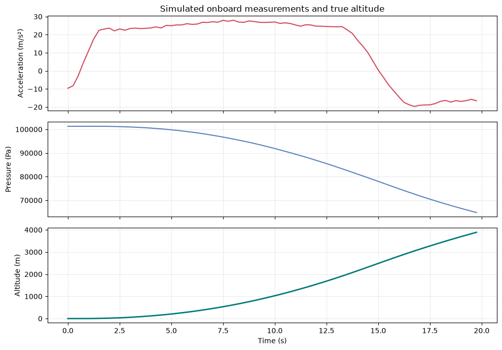
2. The notebook simulates vertical rocket flights with a
physics-based model (thrust, variable mass, gravity, drag, and altitude-dependent atmosphere)
and noisy sensors.
Item
Content
Inputs
X
Shape
(N,


                    2,


                    80)
: accelerometer (m/s²) and barometric pressure (Pa)
Target
y
Shape
(N,


                    80)
: altitude trajectory (m)
Time window
80 samples, one every 0.25 s: 20 s of flight
Splits
Training (700 flights), validation (140), calibration (64), and test (140), generated
independently
Preprocessing
Per-channel standardization, fitted on the training split only, and applied to all
splits
Expected result:
the notebook prints
Input


               shape:


               (700,


               2,


               80)
and
Target


               shape:


               (700,


               80)
, then plots the sensor distributions and one test flight:
Inputs (acceleration and pressure) and target (altitude) of one simulated test flight

Note
The data is
synthetic: realistic enough for learning, but not real flight data. The
calibration split contains inputs only: quantization never uses the labels.
Run notebook section
3. It trains a
tsai FCNPlus
regressor and exports it to ONNX:
Architecture: three 1D convolution blocks (16, 32, and 16 filters; kernel sizes 7, 5,
and 3) without batch normalization, then global average pooling and a linear layer that
predicts the 80 altitude values.
Export: a wrapper converts the normalized outputs back to meters, then
torch.onnx.export writes _tutorial_artifacts/rocket_altitude_tracker_float.onnx
(opset 17, input time_series, output altitude_m).
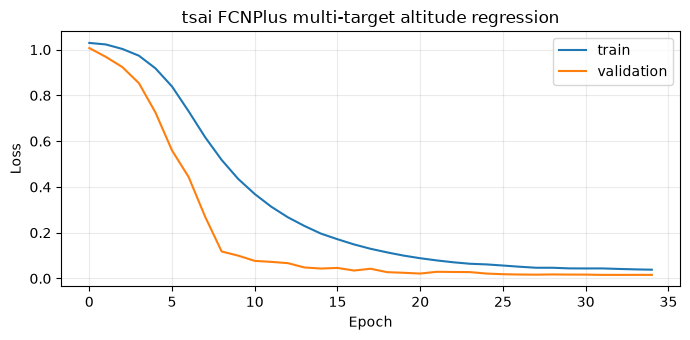
Expected result:
The training and validation losses decrease, then converge:
Run notebook section
4. It starts with a quantization theory recap, then its code cell
builds the configuration with
build_qmn_config()
from
time_series_tutorial_utils.py,
wraps the calibration split in a calibration data reader, and quantizes the float model:
quark_config=build_qmn_config(activation_bits=ACTIVATION_BITS,# 16: W8A16 Qmnadaquant=USE_ADAQUANT,# Truenum_iterations=ADAQUANT_ITERATIONS,# 100 iterations per layer)float_session=ort.InferenceSession(str(FLOAT_MODEL_PATH),providers=["CPUExecutionProvider"])input_name=float_session.get_inputs()[0].namecalibration_reader=NumpyCalibrationDataReader(input_name,X_calibration)quantizer=ModelQuantizer(quark_config)quantizer.quantize_model(str(FLOAT_MODEL_PATH),str(QUANTIZED_MODEL_PATH),calibration_reader,)
Expected result:
the Quark log shows, in this order:
the calibration on 64 samples, with the PowerOfTwoMethod.MinMSE method, in about
10 seconds
a warning that 16-bit QuantizeLinear and DequantizeLinear nodes require ONNX opset
21: as the float model uses opset 17, Quark writes them in the com.microsoft domain,
which ONNX Runtime supports
AdaQuant optimizing the three convolutions and the linear layer (Gemm), 100 iterations
each, in about 1 second
a final table with INT16 activations for all operator types, and INT8 weights for the
convolutions and the Gemm layer
The quantized model is saved as
_tutorial_artifacts/rocket_altitude_tracker_w8a16_qmn.onnx.
Note
For each layer, the AdaQuant log shows two kinds of values:
adaquantiterations=...,loss=...: the loss of one training step, computed on one
calibration sample. This value is noisy: it can increase from one line to the next.
reconsmetricswasoptimizedfromAtoB: the mean squared error of the layer output
on all the calibration samples, before (A) and after (B) AdaQuant. This is the value
to check: B must be lower than A.
Run notebook section
5. It checks the quantized model (ONNX checker, presence of Q/DQ
nodes, finite predictions), then computes regression metrics on the 140 test flights: over
the whole trajectory (
sequence), and at the last time step (
final step).
Expected result
(reference run, see the versions in
Assets):
Metric on 140 test flights
Float ONNX
W8A16 Qmn
Sequence MAE (m)
15.43
18.11
Sequence RMSE (m)
25.23
26.94
Sequence R²
0.9991
0.9989
Final-step MAE (m)
40.71
40.91
Final-step RMSE (m)
51.65
52.49
Final-step R²
0.9913
0.9910
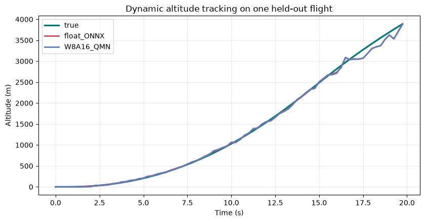
The W8A16 Qmn model keeps R² above 0.99. Its sequence MAE increases by 2.7 m, for final
altitudes between 1157 m and 3889 m.
The mean absolute difference between the float and quantized predictions is 7.2 m
(26.6 m at most).
The quantized model contains 36 Q/DQ nodes.
True altitude versus float and W8A16 Qmn predictions, for the highest test flight

Your values can differ slightly, depending on your platform and package versions.
Comparison with W8A8 Qmn and without AdaQuant.
To measure the benefit of 16-bit
activations and of AdaQuant on this model, set
ACTIVATION_BITS


               =


               8
or
USE_ADAQUANT


               =


               False
in the first code cell of section 1, then run the notebook again.
Reference results on the 140 test flights:
Configuration
Sequence MAE (m)
Maximum difference from the float model (m)
Float ONNX
15.43
—
W8A16 Qmn with AdaQuant
18.11
26.6
W8A16 Qmn without AdaQuant
18.30
36.4
W8A8 Qmn with AdaQuant
20.16
560.3
16-bit activations keep the quantized predictions close to the float model. With
8-bit activations, the worst-case prediction is 560 m away from the float prediction. The
model outputs altitudes in meters, up to about 3900 m: with a power-of-two scale, the
output tensor has a step of 32 m in int8, versus 0.125 m in int16.
AdaQuant reduces the sequence MAE from 18.30 m to 18.11 m, and the maximum difference
from the float model from 36.4 m to 26.6 m, in about 1 second.
To quantize your own time-series regressor with this workflow (see also notebook section
6), prepare:
Inputs shaped (N,C,T): samples, channels, and time steps.
Targets shaped (N,1) for sequence-to-one regression, or (N,T) for trajectory
regression, as in this notebook.
Preprocessing statistics computed on the training split only.
A calibration split of representative inputs, preprocessed like the inference inputs,
and separate from the test set.
Then export the float model to ONNX, quantize it with your calibration inputs, and compare
the float and quantized metrics on held-out data before deployment.
Compare with W8A8 on your model: run the Part 2 script with --activation-bits8, or
set ACTIVATION_BITS=8 in the Part 3 notebook, then compare the accuracy and the
activation memory.
Tune AdaQuant: run the Part 2 script with --no-adaquant or other
--adaquant-iterations values, to measure the effect of AdaQuant on your model.
Editable install fails on Windows with MSVC error C2429: install the fork with
python-mpipinstall--no-build-isolation-e./AMD-Quark. Without
--no-build-isolation, pip builds Quark with the latest PyTorch release, instead of the
PyTorch version of the virtual environment.
Custom operators fail to compile: the log contains
CPUversionofcustomopslibrarycompilationfailed, followed by the cause:
Command'['where','cl']'returnednon-zeroexitstatus1: the C++ compiler is not
on the PATH. Run the command from the x64 Native Tools Command Prompt for VS (see
1. Install the C++ build tools).
NinjaisrequiredtoloadC++extensions: the virtual environment is not activated.
Activate it: Quark installs the ninja build tool in it.
Other compilation errors: in the Visual Studio Installer, check that the Desktop
development with C++ workload includes the MSVC x64/x86 build tools and a
Windows 11 SDK. As an alternative, use WSL.
Quark compiles the custom operators again at the next importquark.onnx.
XInt16Spec import error: ImportError:cannotimportname'XInt16Spec' means that
Python imports another AMD Quark package than the ST fork. Run
python-mpipuninstall-yamd-quark, reinstall the fork with
python-mpipinstall--no-build-isolation-e./AMD-Quark, and check that
python-mpipshowamd-quark prints an Editableprojectlocation in the
AMD-Quark clone.
pip fails behind a corporate proxy, with connection or SSL certificate errors: set the
proxy variables as described in the Set up the proxy and SSL variables section of
How to install the STM32 model zoo. Also upgrade pip with
python-mpipinstall--upgradepip: recent pip versions use the certificate store of
the operating system.
Harmless Quark messages: these messages do not stop the quantization.
The api `activation` has been replaced with `input_tensors`: deprecation notice of
the Quark API used in this tutorial.
“TensorsRangeFile” is deprecated: deprecation notice of an internal Quark option.
The opset version is 17 < 20. Skipping fusing Gelu: the models of this tutorial have
no Gelu activation.
GPU version of custom ops library compilation failed, with a CUDA build of PyTorch
only: quantization runs on CPU.
Opset 21 warning for 16-bit QuantizeLinear and DequantizeLinear, printed twice:
standard ONNX supports 16-bit Q/DQ nodes from opset 21 only. With an older opset, Quark
writes them in the com.microsoft domain, which ONNX Runtime runs. If your downstream
tool requires standard ONNX Q/DQ nodes, quantize a float model exported with opset 21 or
later.
ONNX Runtime error during the Part 2 evaluation: Gotinvaliddimensionsforinput
means that the test batch does not match the model input. If the batch dimension of the
model is fixed, run the script with --batch-size1. Also check --input-size and the
NCHW layout.
Large accuracy drop after quantization: check, in this order:
The float accuracy, measured with --float-only (Part 2), matches the expected
accuracy of the model. Otherwise, the preprocessing or the class order is wrong.
The calibration and evaluation preprocessing match the training preprocessing (color
order, resize, and normalization).
The test sub-folder order matches the class order used for training (Part 2).
The calibration data is representative of the deployment data, and not taken from the
test set.
AdaQuant is enabled. Try more iterations, or more calibration samples.
Memory error during the Part 2 calibration: the script keeps all calibration images in
memory. Reduce the number of calibration images.
time_series_tutorial_utils.py was not found (Part 3): copy the helper module next to
the notebook, and start Jupyter from that folder.
Datasets — Part 2: Flowers,
3670 photos under the CC BY 2.0 license (the LICENSE.txt file of the dataset archive
credits the photographers). Part 3: synthetic data, generated by the notebook.
The tutorial scripts, notebook, and helper module are provided under the BSD-3-Clause
license. The Part 2 float model is provided under the SLA0044 license. The reference results
were obtained on Windows 11 with Python 3.13, ONNX 1.21.0, ONNX Runtime 1.25.1, PyTorch 2.7.1,
torchvision 0.22.1, tsai 0.4.1, and AMD Quark 0.12.post1 (ST fork, commit
9d632d9).

 general